DDPM Paper Learning Note
Learning Motivation
Recently, AI model has a great impact on the field of art. The drawing bot “Midjourney” is performing impressivly. With a simple text input, the model will generate an image that fits our need very well. Therefore, I want to figure out what is the logic behind this generation process.
Following is an interesting sample that generated by “Midjourney”:
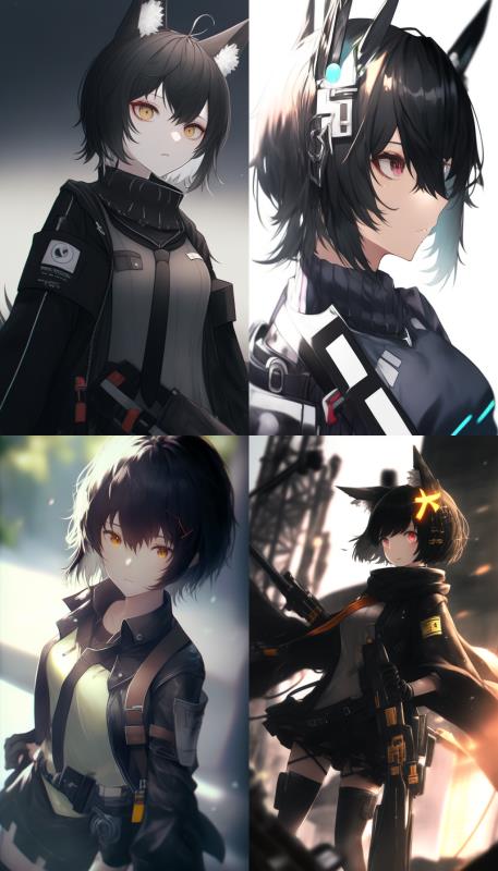
Keywords: pixiv, arknights, girl, black hair, short hair, ultra-detailed, high quality, 4k –ar 4:7 –stop 90 –upbeta –niji
2.Background
There are 3 papers I found which are related to this topic.
-
Deep unsupervised learning using nonequilibrium thermodynamics (2015) by Jascha Sohl-Dickstein, Eric Weiss, Niru Maheswaranathan, and Surya Ganguli.
-
Denoising Diffusion Probabilistic Models (2020) by Jonathan Ho, Ajay Jain, Pieter Abbeel
-
Hierarchical Text-Conditional Image Generation with CLIP Latents (2022) by Aditya Ramesh, Prafulla Dhariwal, Alex Nichol, Casey Chu, Mark Chen
I will briefly introduce them in the following sections.
2.1 Deep unsupervised learning using nonequilibrium thermodynamics (2015)
In this paper, the author manage to Destory the data by diffusion, and then learn a reverse diffusion process that restores structure in data, yielding a highly flexible and tractable generative model of the data.
- Historically, probabilistic models suffer from a tradeoff between two conflicting objectives: tractability and flexibility. Models that are tractable can be analytically evaluated and easily fit to data (e.g. a Gaussian or Laplace). However, these models are unable to aptly describe structure in rich datasets On the other hand, models that are flexible can be molded to fit structure in arbitrary data.
Now here comes a problem. It is possible to learn a model p to reverse the diffusion process so that we can share the benifit of both tractability and flexibility?
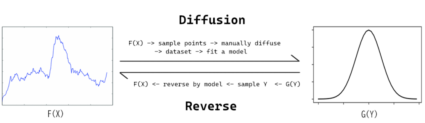
Combining the concepts from Theromodynamics and Maching Learning, the authors of this paper successfully find a flexible and tractable model to reverse the diffusion process. But unfortunally, there is no evidence showing that this model is capable of high quality image generation, which leave some works for the later researchers.
2.2 Denoising Diffusion Probabilistic Models (2020)
This paper (known as the DDPM paper) successfully shows that the diffusion probabilistic model is capable to generate high quality images.Here is what they said:
- Diffusion models are straightforward to define and efficient to train, but to the best of our knowledge, there has been no demonstration that they are capable of generating high quality samples. We show that diffusion models actually are capable of generating high quality samples, sometimes better than the published results on other types of generative models.
Several changes has been made by the authors of DDPM to the original version of diffusion model.
- Apply a linearly increasing diffusion rate schedule \(\beta_{1:T}\). to the diffusion process.
- Only add Gaussian noise to each step of diffusion.
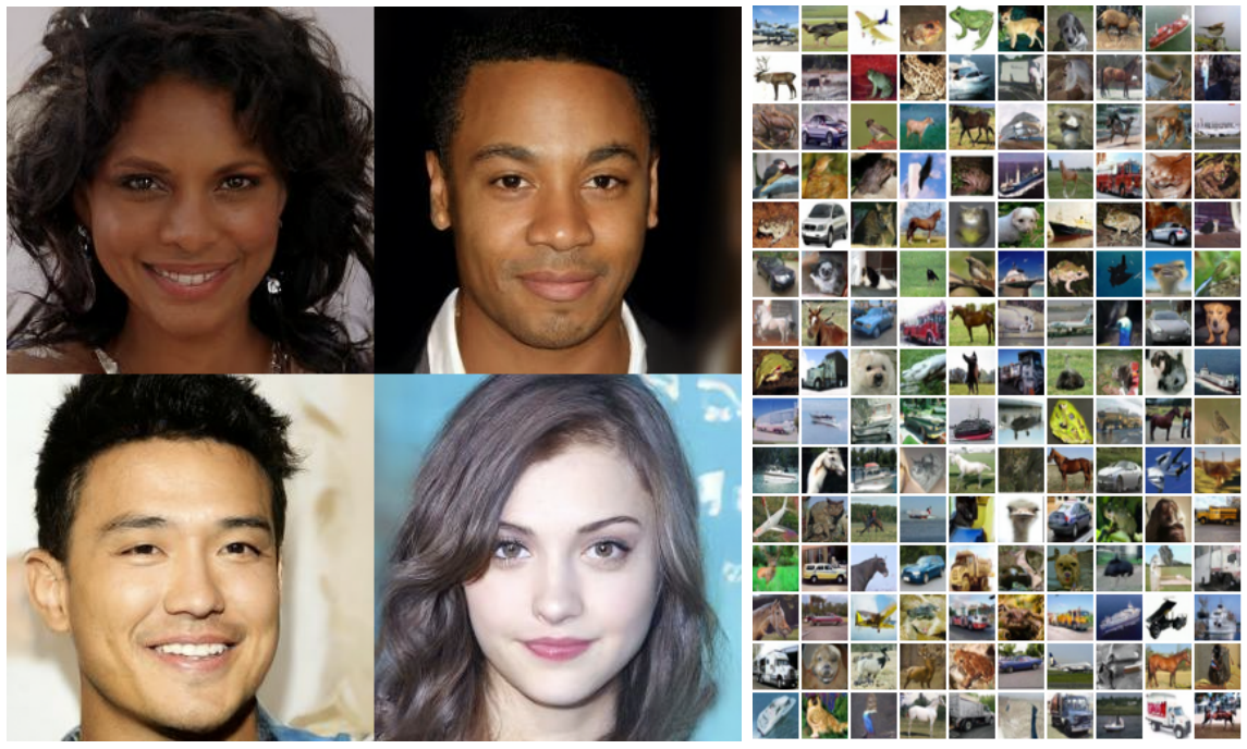
The following are some images that generated by the modified diffusion model, which is trained by CelebA-HQ 256 × 256 (left) and unconditional CIFAR10 (right):
2.3 Hierarchical Text-Conditional Image Generation with CLIP Latents (2022)
This is a paper for the well-known OpenAI project “DALL-E2”. Even though the we don’t know what model “Midjourney” is using, we can fairly predict that they are using the similar model like “DALL-E2” because the input and output of them are similar.
The following is the architacture of the “DALL-E2” model.
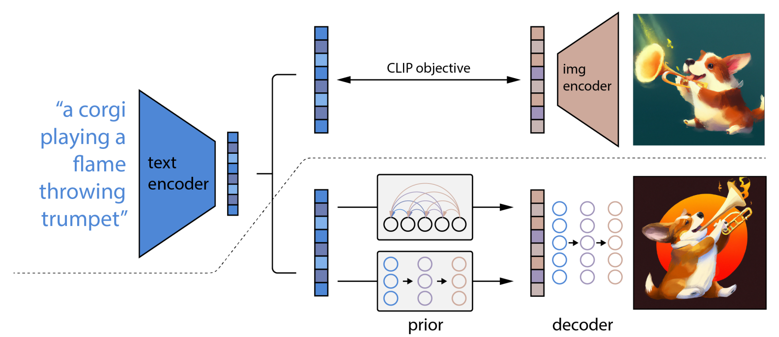
- A high-level overview of unCLIP. Above the dotted line, we depict the CLIP training process, through which we learn a joint representation space for text and images. Below the dotted line, we depict our text-to-image generation process: a CLIP text embedding is first fed to an autoregressive or diffusion prior to produce an image embedding, and then this embedding is used to condition a diffusion decoder which produces a final image. Note that the CLIP model is frozen during training of the prior and decoder
My study will only focus on the diffusion model part base on the DDPM paper.
3.Derivation of Diffusion Model
In this section, I will follow the idea of the DDPM paper and do the derivation of the diffusion model untill we get the final loss function.
3.1 Diffusion Process
- Objective: Find an easy way to get \(X_{t}\) directly from \(X_{0}\)
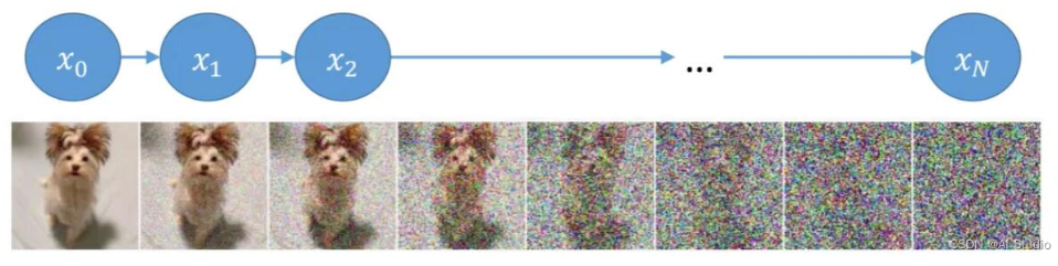
The image above is the diffusion process. Intuitively, the diffusion process just simply add noise to the image over and over again and finally get a image that follows a standard Gaussian distribution.
Base on the setup of the DDPM paper, the diffusion process will have a fix linear schedule diffusion rate and only add gaussian noise for each diffusion. More specifically, we have:
\[q(X_t|X_{t-1}) = \mathcal{N}(X_{t}; \sqrt{\alpha_t}X_{t-1}, (1-\alpha_t) \textbf{I})\]Therefore, there is a recursive relation to the \(X_{t}\) and \(X_{t-1}\), which is:
\[X_t = \sqrt{\alpha_t} X_{t-1} + \sqrt{1 - \alpha_t}\epsilon_t, \epsilon_t \sim \mathcal{N}(0,\textbf{I})\]Naively, we can get any \(X_{t}\) recursively from \(X_{0}\), but it is not efficient. Therefore, we will try to find a general form.
We can replace \(X_{t-1}\) with the recursive formular and see what we will get:
\[\begin{aligned} X_t &= \sqrt{\alpha_t} X_{t-1} + \sqrt{1 - \alpha_t}\epsilon_t \\ &= \sqrt{\alpha_t} (\sqrt{\alpha_{t-1}} X_{t-2} + \sqrt{1 - \alpha_{t-1}}\epsilon_{t-1}) + \sqrt{1 - \alpha_t}\epsilon_t \\ &= \sqrt{\alpha_t \alpha_{t-1}} X_{t-2} + \sqrt{\alpha_t - \alpha_t \alpha_{t-1}}\epsilon_{t-1} + \sqrt{1-\alpha_t}\epsilon_t \end{aligned}\]The coefficient of \(X_{t-2}\) is simple, but how to deal with the remaining two components? Recall that \(\epsilon_{t-1}\) and \(\epsilon_{t}\) are both following the standard Gaussian. Therefore, we have:
\[\sqrt{\alpha_t - \alpha_t \alpha_{t-1}}\epsilon_{t-1} \sim \mathcal{N}(0,(\alpha_t - \alpha_t \alpha_{t-1})\textbf{I})\] \[\sqrt{1-\alpha_t}\epsilon_t \sim \mathcal{N}(0,(1-\alpha_t)\textbf{I})\]Which means that we can combine the two noise in the following way:
\[\begin{aligned} X_t &= \sqrt{\alpha_t \alpha_{t-1}} X_{t-2} + \sqrt{\alpha_t - \alpha_t \alpha_{t-1}}\epsilon_{t-1} + \sqrt{1-\alpha_t}\epsilon_t\\ &=\sqrt{\alpha_t \alpha_{t-1}} X_{t-2} + \sqrt{1 - \alpha_t \alpha_{t-1}}\epsilon \end{aligned}\]Then, we can do the same thing for T-1 times and we will get the following:
\[\begin{aligned} X_t&=\sqrt{\alpha_t \alpha_{t-1} \dots \alpha_{1}} X_{0} + \sqrt{1 - \alpha_t \alpha_{t-1} \dots \alpha_{1}}\epsilon\\ &= \sqrt{\overline{\alpha}_t} X_{0} + \sqrt{1 -\overline{\alpha}_t}\epsilon \end{aligned}\]Meaning that:
\[X_t \sim \mathcal{N}(X_t; \sqrt{\overline{\alpha}_t}X_0, (1-\overline{\alpha_t})\textbf{I})\] \[q(X_t|X_0) = \mathcal{N}(X_t; \sqrt{\overline{\alpha}_t}X_0, (1-\overline{\alpha_t})\textbf{I})\]So far, the forward diffusion process is completely known by us because we can get any distribution of the middle state as long as we want.
The next step is to figure out the distribution of the reverse process for the sake of training the reverse model.
3.2 Reverse Process
-
Objective: Find \(q(X_{t-1} X_{t})\)
Using the Bayes Theorem, we can transfor the reverse distribution to the combination of forward distribution:
\[\begin{aligned} q(X_{t-1}|X_t,X_0) &= \frac{q(X_t|X_{t-1},X_0)q(X_{t-1}|X_0)}{q(X_{t}|X_0)} \end{aligned}\]Form the forward process analysis, we know that:
\[q(X_t|X_{t-1},X_0) \sim \mathcal{N}(X_{t}; \sqrt{\alpha_t}X_{t-1}, (1-\alpha_t) \textbf{I})\] \[q(X_{t-1}|X_0) \sim \mathcal{N}(X_{t-1}; \sqrt{\overline{\alpha}_{t-1}}X_{0}, (1-\overline{\alpha}_{t-1}) \textbf{I})\] \[q(X_{t}|X_0) \sim \mathcal{N}(X_{t}; \sqrt{\overline{\alpha}_t} X_{0}, (1-\overline{\alpha}_t) \textbf{I})\]Replace them with the Gaussian expression, we will have:
\[\begin{aligned} &q(X_{t-1}|X_t,X_0) \\ &= \frac{q(X_t|X_{t-1},X_0)q(X_{t-1}|X_0)}{q(X_{t}|X_0)}\\ &\propto exp(-\frac{1}{2}( \frac{(X_t - \sqrt{\alpha_t}X_{t-1})^2}{1-\alpha_t} + \frac{(X_{t-1} - \sqrt{\overline{\alpha}_t}X_{0})^2}{1-\overline{\alpha}_{t-1}} - \frac{(X_t - \sqrt{\overline{\alpha}_t}X_{0})^2}{1-\overline{\alpha}_{t}}))\\ &= exp(-\frac{1}{2}( \frac{X_t^2 - 2\sqrt{\alpha_t}X_t X_{t-1} + \alpha_tX_{t-1}^2}{1-\alpha_t} + \frac{X_{t-1}^2 - 2\sqrt{\overline{\alpha}}_{t-1}X_{0} X_{t-1} + \overline{\alpha}_{t-1} X_{0}^2}{1-\overline{\alpha}_{t-1}}-\frac{(X_t - \sqrt{\overline{\alpha}_t}X_{0})^2}{1-\overline{\alpha}_{t}})\\ &= exp(-\frac{1}{2}( (\frac{\alpha_t}{1- \alpha_t} + \frac{1}{1- \overline{\alpha}_{t-1}})X_{t-1}^2 - (\frac{2\sqrt{\alpha_t}}{1-\alpha_t}X_{t} + \frac{2\sqrt{\overline{\alpha}_{t-1}}}{1-\overline{\alpha}_{t-1}}X_0)X_{t-1} + C(X_t,X_0) )) \end{aligned}\]Be aware that we are looking for the distribution over \(X_{t-1}\), which means that our goal is to find the mean and varient of it. Now, recall the basic form of a Gaussian distribution:
\[exp(-\frac{(x-\mu)^2}{2\sigma^2}) = exp(-\frac{1}{2}(\frac{1}{\sigma^2}x^2 - \frac{2\mu}{\sigma^2}x + \frac{\mu^2}{\sigma^2}))\]Compare those two formular, we can have the following equation to solve the mean and varient:
\[\begin{cases} \frac{1}{\sigma_t^2} = \frac{\alpha_t}{1- \alpha_t} + \frac{1}{1- \overline{\alpha}_{t-1}}\\ \frac{2\tilde{\mu}_{t}(X_t,X_0)}{\sigma_t^2} = \frac{2\sqrt{\alpha_t}}{1-\alpha_t}X_{t} + \frac{2\sqrt{\overline{\alpha}_{t-1}}}{1-\overline{\alpha}_{t-1}}X_0\\ X_t = \sqrt{\overline{\alpha}_t} X_{0} + \sqrt{1 -\overline{\alpha}_t}\epsilon \end{cases}\]Therefore,
\[\begin{cases}\tilde{\mu}_{t}(X_t,X_0) = \frac{1}{\sqrt{\alpha_t}} (X_t - \frac{1-\alpha_t}{\sqrt{1-\overline{\alpha}_t}}\epsilon_t)\\ \sigma_t^2 = \frac{(1-\alpha_t)(1-\overline{\alpha}_{t-1})}{1-\alpha_t\overline{\alpha}_{t-1}}\end{cases}\]So far, we have got the distribution of the reverse process. Next step is to figure out a way to train the reverse model.
3.3 Training
Before we start working with the loss function, we need to understand “KL divergence”:
- KL divergence compares two different distribution.
- KL divergence lower bounded by 0
Supposed we have two pdf function f(x) and g(x), the KL divergence between then should be:
\[\begin{aligned} D_{KL}(f(x)||g(x)) &= \int f(x) \log(\frac{f(x)}{g(x)})dx\\ &= - \int f(x) \log(\frac{g(x)}{f(x)}) dx\\ & \ge - \int f(x) (\frac{g(x)}{f(x)} - 1) dx\\ &= - \int g(x) - f(x) dx\\ &= 0 \end{aligned}\]Now, we have a way to compare two distribution. Recall that we want the trained model able to generate a distribution\(p_{\theta}(X’)\) which is as close as the original dataset distribution \(q(X)\). Therefore, we can use the KL divergence between those two distribution as our objective:
\[\begin{aligned} D_{KL}(q(X_0)||p_{\theta}(X_0)) &= \int q(X_0) \log[\frac{q(X_0)}{p_{\theta}(X_0)}]d(X_0)\\ &= \int q(X_0) \log[q(X_0)]d(X_0) - \int q(X_0) \log[p_{\theta}(X_0)]d(X_0)\\ &= - \mathcal{H}(q(X_0)) + \mathcal{H}(q(X_0), p_{\theta}(X_0)) \end{aligned}\]Because \(q(X_0)\) is a distribution of dataset, it is fixed, so as its entropy \(\mathcal{H}(q(X_0))\), to minimize the given kl divergence, we just need to deal with the cross entropy \(\mathcal{H}(q(X_0), p_{\theta}(X_0))\).
\[\begin{aligned} \mathcal{H}(q(X_0), p_{\theta}(X_0)) &= - \int q(X_0)\log[p_{\theta}(X_0)]d(X_0)\\ &= - \mathbb{E}_{q(X_0)} \log p_{\theta}(X_0)\\ &= -\mathbb{E}_{q(X_0)}\log [\int p_{\theta}(X_{0:T}) d(X_{1:T})]\\ &= -\mathbb{E}_{q(X_0)}\log [\int q(X_{1:T} | X_0) \frac{p_{\theta}(X_{0:T})}{ q(X_{1:T} | X_0)} d(X_{1:T})]\\ &= -\mathbb{E}_{q(X_0)} \log[\mathbb{E}_{q(X_{1:T}| X_0)}\frac{p_{\theta}(X_{0:T})}{ q(X_{1:T} | X_0)}] \end{aligned}\]Recall the Jensen’s inequality. For any convex function, we have:
\[\mathcal{\varphi}[\mathbb{E}(X)] \leq \mathbb{E}[\mathcal{\varphi}(X)]\]Here, we will apply the Jensen’s inequality to find the upper bound of this cross entropy:
\[\begin{aligned} \mathcal{H}(q(X_0), p_{\theta}(X_0)) &= -\mathbb{E}_{q(X_0)} \log[\mathbb{E}_{q(X_{1:T}| X_0)}\frac{p_{\theta}(X_{0:T})}{ q(X_{1:T} | X_0)}]\\ & \leq -\mathbb{E}_{q(X_0)} \mathbb{E}_{q(X_{1:T}| X_0)}\log[\frac{p_{\theta}(X_{0:T})}{ q(X_{1:T} | X_0)}]\\ &= -\mathbb{E}_{q(X_{0:T})} \log[\frac{p_{\theta}(X_{0:T})}{ q(X_{1:T} | X_0)}]\\ &= \mathbb{E}_{q(X_{0:T})} [\log\frac{ q(X_{1:T} | X_0)}{p_{\theta}(X_{0:T})}]\\ \end{aligned}\]Since the upper bound is still a join distribution, not friendly enough, we use the Morkov chain property and keep moving forward:
\[\begin{aligned} & \mathbb{E}_{q(X_{0:T})} [\log\frac{ q(X_{1:T} | X_0)}{p_{\theta}(X_{0:T})}] \\ &= \mathbb{E}_{q} [\log\frac{\Pi_{t=1}^{T}q(X_t|X_{t-1})}{p_{\theta}(X_T)\Pi_{t=1}^{T}p_{\theta}(X_{t-1} | X_t)}]\\ &= \mathbb{E}_{q} [-\log p_{\theta}(X_T) + \sum_{t=1}^{T}\log\frac{q(X_t|X_{t-1})}{p_{\theta}(X_{t-1} | X_t)}]\\ &= \mathbb{E}_{q} [-\log p_{\theta}(X_T) + \sum_{t=2}^{T}\log\frac{q(X_t|X_{t-1})}{p_{\theta}(X_{t-1} | X_t)} + \log \frac{q(X_1|X_0)}{p_{\theta}(X_0 | X_1)}]\\ &= \mathbb{E}_{q} [-\log p_{\theta}(X_T) + \sum_{t=2}^{T}\log(\frac{q(X_{t-1}|X_t, X_0)}{p_{\theta}(X_{t-1} | X_t)} \frac{q(X_t|X_0)}{q(X_{t-1}|X_0)}) + \log \frac{q(X_1|X_0)}{p_{\theta}(X_0 | X_1)}]\\ &= \mathbb{E}_{q} [-\log p_{\theta}(X_T) + \sum_{t=2}^{T}\log\frac{q(X_{t-1}|X_t, X_0)}{p_{\theta}(X_{t-1} | X_t)} + \sum_{t=2}^{T}\log \frac{q(X_t|X_0)}{q(X_{t-1}|X_0)} + \log \frac{q(X_1|X_0)}{p_{\theta}(X_0 | X_1)}]\\ &= \mathbb{E}_{q} [-\log p_{\theta}(X_T) + \sum_{t=2}^{T}\log\frac{q(X_{t-1}|X_t, X_0)}{p_{\theta}(X_{t-1} | X_t)} + \log \frac{q(X_T|X_0)}{q(X_1|X_0)} + \log \frac{q(X_1|X_0)}{p_{\theta}(X_0 | X_1)}]\\ &= \mathbb{E}_{q} [-\log p_{\theta}(X_T) + \sum_{t=2}^{T}\log\frac{q(X_{t-1}|X_t, X_0)}{p_{\theta}(X_{t-1} | X_t)} + \log \frac{q(X_T|X_0)}{p_{\theta}(X_0 | X_1)}]\\ &= \mathbb{E}_{q} [\log \frac{q(X_T|X_0)}{p_{\theta}(X_T)} + \sum_{t=2}^{T}\log\frac{q(X_{t-1}|X_t, X_0)}{p_{\theta}(X_{t-1} | X_t)} - \log p_{\theta}(X_0 | X_1)]\\ &= \mathbb{E}_{q} [\begin{matrix} \underbrace{D_{KL}(q(X_T|X_0)||p_{\theta}(X_T))} \\ L_T \end{matrix} + \begin{matrix} \underbrace{\sum_{t=2}^{T} D_{KL}(q(X_{t-1}|X_t, X_0)||p_{\theta}(X_{t-1} | X_t)) } \\ L_{T-1 : 1} \end{matrix} + \begin{matrix} \underbrace{- \log p_{\theta}(X_0 | X_1)}\\ L_{0} \end{matrix}] \end{aligned}\]Now the upper bound of the crocess entropy can be written as:
\[\mathcal{H}(q(X_0), p_{\theta}(X_0)) \leq L_T + L_{T-1} + L_{T-2} + \dots + L_0\]where:
\[\begin{aligned} L_T &= D_{KL}(q(X_T|X_0)||p_{\theta}(X_T))\\ L_{t-1} &= D_{KL}(q(X_{t-1}|X_t, X_0)||p_{\theta}(X_{t-1} | X_t)), 2 \leq t \leq T\\ L_{0} &= - \log p_{\theta}(X_0 | X_1)\\ \end{aligned}\]For \(L_T\), recall that \(p_{\theta}(X_T))\) is a standard Gassian, it has nothing to do with \(\theta\).Therefore, we don’t need to put it into consideration.
For \(L_0\), it is the final step of the reverse process of the generative model, we can treat it as a decoder to decode \(X_1\) to \(X_0\). We can sample it from a Gaussian distribution \(\mathcal{N}(X_{0}; \mu_{\theta}(X_1,1), \sigma_{1}^2 \textbf{I})\) after we trained a model.
Therefore, our goal is to minimize \(L_{1 : T-1}\) so as to minimize the upper bound of the cross entropy.
\(L_{1 : T-1}\) is the KL divergence of the two reverse distributions between the one get from the dataset \(q(X_T|X_0)\) and the one generated by the model \(p_{\theta}(X_T)\).
Because they are both Gaussian distribution with the same varience, we can compare their mean. The loss function can be written as:
\[\begin{aligned} \mathcal{L}_t &= \mathbb{E}_{X_0,\epsilon}[ \frac{1}{2||\Sigma_{\theta}(X_t,t)||_2^2} ||\tilde{\mu}_t(X_t, X_0) - \mu_{\theta}(X_t,t)||^2 ]\\ &= \mathbb{E}_{X_0,\epsilon}[ \frac{1}{2||\Sigma_{\theta}(X_t,t)||_2^2} ||\frac{1}{\sqrt{\alpha_t}} (X_t - \frac{1-\alpha_t}{\sqrt{1-\overline{\alpha}_t}}\epsilon_t) - \frac{1}{\sqrt{\alpha_t}} (X_t - \frac{1-\alpha_t}{\sqrt{1-\overline{\alpha}_t}}\epsilon_{\theta}(X_t,t))||^2 ]\\ &= \mathbb{E}_{X_0,\epsilon}[ \frac{\beta_t^2}{2\alpha_t(1-\overline{\alpha}_t)||\Sigma_{\theta}||^2_2} ||\epsilon_t - \epsilon_{\theta}(X_t,t)||^2 ]\\ &= \mathbb{E}_{X_0,\epsilon}[ \frac{\beta_t^2}{2\alpha_t(1-\overline{\alpha}_t)||\Sigma_{\theta}||^2_2} ||\epsilon_t - \epsilon_{\theta}(\sqrt{\overline{\alpha}_t} X_0 + \sqrt{1- \overline{\alpha}_t}\epsilon_t,t)||^2 ]\\ \end{aligned}\]Here, we use the reparameterization trick in the loss function, which transfer the training variable from \(\mu_{\theta}\) to \(\epsilon_{\theta}\).
The reason to do that is quite straight forward. It has a better training result.
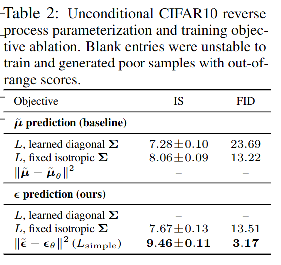
We can see that, overall, the IS score is greater and the FDI score is smaller when we train over \(\epsilon_{\theta}\).
Furthermore, in the phesis paper itself, it has the following statement to further explain the reason:
- We have shown that the є-prediction parameterization both resembles Langevin dynamics and simplifies the diffusionmodel’s variational bound to an objective that resembles denoising score matching.
Finally, we have a loss function, then we need to wrap up and find an algorithm to actually do our training.
This algorithm has two saperate part, Training and Sampling.

For the Training part, we will sample several images from the dataset and do diffusion over them. The time schedule t will randomly sample from a Uniform distribution so that we are able to have a datase with different diffusion step for the model to learn. After the training, the model will be able to generate any \(\epsilon_{t}\) given \(X_{t}\) and t.
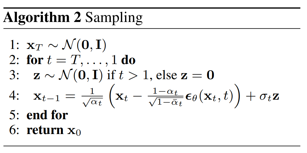
For the Sampling part, we can make use of the trained model to get any noise that we added to step t, so that we can calculate the step t-1 image with the formular we get from the reverse process analysis. Do it for many times, we will finally get an image that higely follow the original distribution of the dataset.
Congratulations! we have derived the loss function of the magical diffusion model!
4.Summery of Derication
Now, let’s briefly overview what we have done:
- Diffusion process: Figure out the expression of \(q(X_t | X_0)\) , the general term formula.
- Reverse process: Figure out the expression of \(q(X_{t-1}| X_{t}, X_0)\).
- Training:
- Objective: Find \(p_{\theta}(X_0)\) as close as \(q(X_0)\)
- Steps:
- Minimize \(D_{KL}(q(X_0)||p_{\theta}(X_0))\)
- Minimize \(\mathcal{H}(q(X_0), p_{\theta}(X_0))\)
- Jensen’s inequality, find the upper bound.
- \(\mathcal{H}(q(X_0), p_{\theta}(X_0))\) bounded by \(\sum_{t=0}^T L_{t}\) which is the sum of \(D_{KL}\)
- Minimize \(D_{KL}(q(X_{t-1}|X_t, X_0)||p_{\theta}(X_{t-1} | X_t))\), which is the same to minimize the difference of mean.
- Do reparameterization to loss function and train the model over the noise variable \(\epsilon\).
- Train the model and use the model to generate image from pure standard Gaussian noise.
5.Experiements
In the section, I will share some of the results of the experiements they did in the DDPM paper.
- Basic setup:
- Set T = 1000 for all experiments, meaning we will diffuse at most 1000 times.
- Set the forward process variances to constants increasing linearly from \(\beta_1 = 10^{-4}\) to \(βT = 0.02\). Making sure that \(D_{KL}(q(X_{t-1}|X_t, X_0)||p_{\theta}(X_{t-1} | X_t))\)
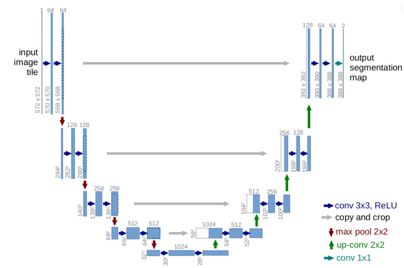
- Using Unet as the architacture of the training model.
Unet is a encoder and decoder using Convolutional neural network architecture. The special point of this structure is that it includes four Skip connections which can carry the original feature from the encoder to the decoder in the same level.
- Comparison between p(x) and q(x’)
This experiement using LSUN dataset, which includes several classes of 256 * 256 image. The following image shows the FID score between the dataset distribution and the generated distribution.
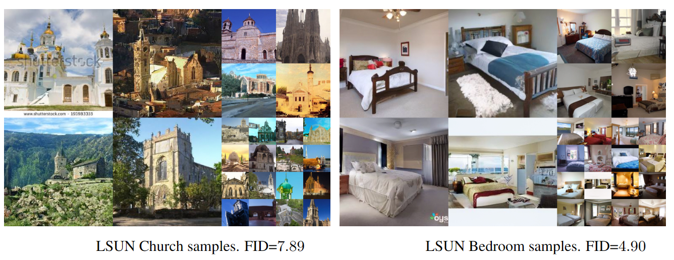
The FID scores of the model are 7.89 on Church datas and 4.90 on Bedroom datas, which is low enough to show how similar the generated distribution and the original distribution is.
- Prograssive Generation
- model was trained on CIFAR10 dataset.
- The leftmost are samples from
- The rightmost are images that generated by the trained model.
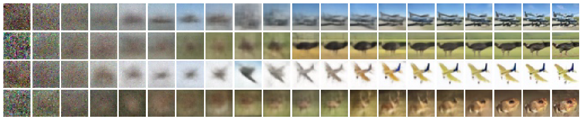
This result shows us the middle states of the generative process, from which we can have a clear view of how the noise is being removed step by step.
- Reverse from different steps of diffusion.
- Using CelebA-HQ 256 × 256 dataset
- For each set, the one from bottom right is the diffused image.
- The other three are generated from the model given the bottom right one.
- The diffused image of each set has different time of diffusion.
- From left to right, the times of diffusion for the diffused images are :T=1000, 750, 500 250, 0.
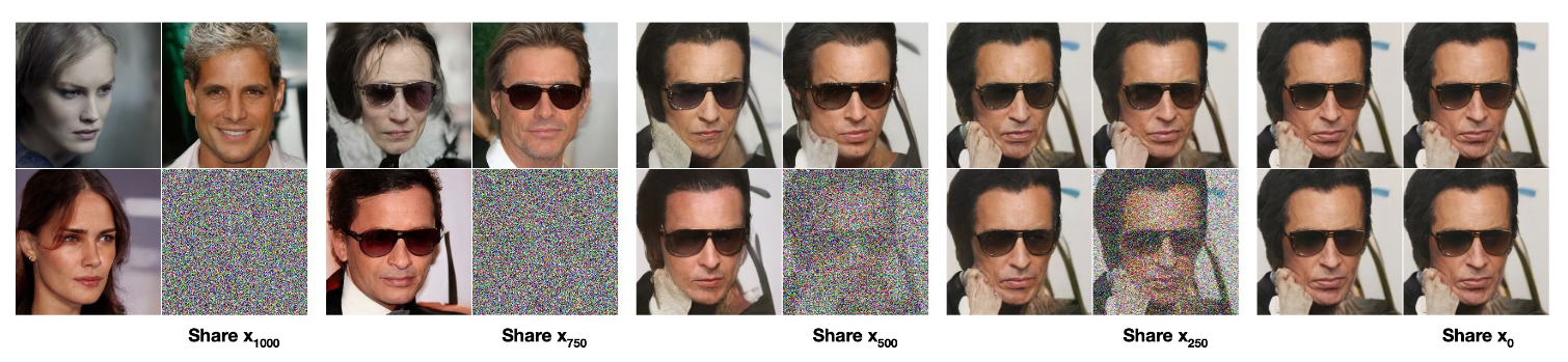
This experiements actually shows the high IS score in a visiable way. When given a more specific input (other than a pure Gaussian noise), the more accuate the model can generate.
- My training result
- Dataset: Fashion-MNIST
- Code reference: https://huggingface.co/blog/annotated-diffusion (This excellent blog also includes good explainations for all the codes.)
- You can play with the code in google colab (The training only take about 10 minute if suing the colab GPU):
![]()
This GIF shows us how the trained diffusion model generates an image that related to Fashion-MNIST distribution from a pure Gaussian noise.

6.Impressive Application
-
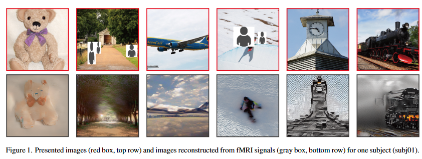
High-resolution image reconstruction with latent diffusion models from human brain activity (2023)
by Yu Takagi, Shinji Nishimoto
This paper from Osaka University shows us a megical algorithm, read our mind! The first row image represents what we are seeing, the second row represents the image that generated by the model with our brain signal.
7.Conclusion and Thinkings
With the help of the diffusion model, we are able to represent a whole dataset distribution only by a train model. Just like we can represent all the points in a line with a single linear equation. We can easily sample from any distribution by passing a Gaussian noise to a model that trained by this data distribution samples.
Possible Future works:
-
Is the face changing implemented with diffusion model by inputing not a pure Gaussian noise but an original image of a face?
-
It is possible to use diffusion model in other area? Not only limited on image but some other things like filling up missing values or dealing with some other data type like voice or text.
-
How to distinguish the image that generated by diffusion model? What moral problems it will cause in the future?
8.Reference
- arXiv:2204.06125 [cs.CV] https://doi.org/10.48550/arXiv.2204.06125
- arXiv:1503.03585 [cs.LG] https://doi.org/10.48550/arXiv.1503.03585
- arXiv:2006.11239v2 [cs.LG] https://doi.org/10.48550/arXiv.2006.11239
- Weng, Lilian. (Jul 2021). What are diffusion models? Lil’Log. https://lilianweng.github.io/posts/2021-07-11-diffusion-models/
- Niels, Rogge. Kashif,RasulThe. Annotated Diffusion Model. https://huggingface.co/blog/annotated-diffusion
- https://aistudio.baidu.com/aistudio/projectdetail/4867936